Plot the overlap via propensity score method
Source:R/plot_overlap_pScores.R
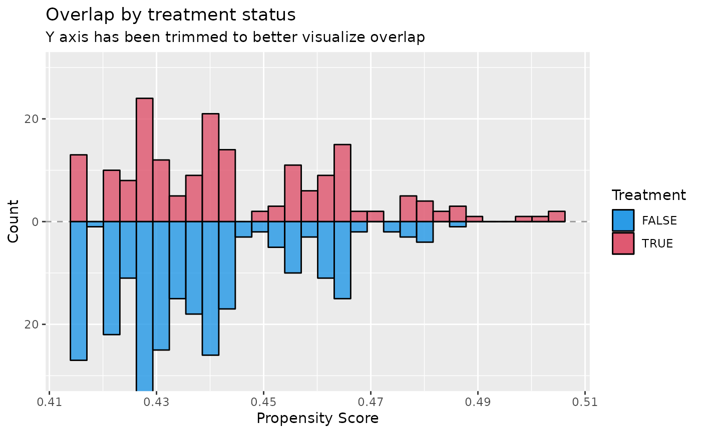
plot_overlap_pScores.RdPlot histograms showing the overlap between propensity scores by treatment status.
Usage
plot_overlap_pScores(
  .data,
  treatment,
  confounders,
  plot_type = c("histogram", "density"),
  trim = TRUE,
  min_x = NULL,
  max_x = NULL,
  pscores = NULL,
  ...
)
Arguments
- .data
dataframe
- treatment
character. Name of the treatment column within .data
- confounders
character list of column names denoting confounders within .data
- plot_type
the plot type, one of c('Histogram', 'Density')
- trim
a logical if set to true y axis will be trimmed to better visualize areas of overlap
- min_x
numeric value specifying the minimum propensity score value to be shown on the x axis
- max_x
numeric value specifying the maximum propensity score value to be shown on the x axis
- pscores
propensity scores. If not provided, then propensity scores will be calculated using BART
- ...
additional arguments passed to `dbarts::bart2` propensity score calculation
Examples
# \donttest{
data(lalonde)
plot_overlap_pScores(
 .data = lalonde,
 treatment = 'treat',
 confounders = c('age', 'educ'),
 plot_type = 'histogram',
 pscores = NULL,
 seed = 44
)
#>
#> Running BART with binary y
#>
#> number of trees: 75
#> number of chains: 4, number of threads 2
#> tree thinning rate: 1
#> Prior:
#> 	prior on k: chi with 1.250000 degrees of freedom and inf scale
#> 	power and base for tree prior: 2.000000 0.950000
#> 	use quantiles for rule cut points: false
#> 	proposal probabilities: birth/death 0.50, swap 0.10, change 0.40; birth 0.50
#> data:
#> 	number of training observations: 445
#> 	number of test observations: 0
#> 	number of explanatory variables: 2
#>
#> Cutoff rules c in x<=c vs x>c
#> Number of cutoffs: (var: number of possible c):
#> (1: 100) (2: 100)
#> Running mcmc loop:
#> [1] iteration: 100 (of 500)
#> [2] iteration: 100 (of 500)
#> [1] iteration: 200 (of 500)
#> [2] iteration: 200 (of 500)
#> [1] iteration: 300 (of 500)
#> [2] iteration: 300 (of 500)
#> [1] iteration: 400 (of 500)
#> [2] iteration: 400 (of 500)
#> [1] iteration: 500 (of 500)
#> [2] iteration: 500 (of 500)
#> [4] iteration: 100 (of 500)
#> [3] iteration: 100 (of 500)
#> [4] iteration: 200 (of 500)
#> [3] iteration: 200 (of 500)
#> [4] iteration: 300 (of 500)
#> [3] iteration: 300 (of 500)
#> [4] iteration: 400 (of 500)
#> [3] iteration: 400 (of 500)
#> [4] iteration: 500 (of 500)
#> [3] iteration: 500 (of 500)
#> total seconds in loop: 0.494210
#>
#> Tree sizes, last iteration:
#> [1] 2 3 2 2 2 2 3 2 2 2 2 2 2 2 3 3 5 2
#> 3 3 2 2 2 1 2 2 2 3 2 2 2 3 4 2 2 4 2 2
#> 2 3 2 1 4 2 2 3 3 2 2 2 3 2 2 3 3 2 3 2
#> 2 2 3 3 2 3 3 2 2 1 2 2 2 4 2 2 2
#> [2] 2 2 2 2 2 2 4 2 2 2 1 2 3 3 2 2 2 2
#> 2 2 2 2 3 2 3 2 2 3 2 2 2 2 3 2 3 4 2 3
#> 3 2 2 2 2 2 3 2 2 2 2 3 3 3 2 2 3 2 2 3
#> 2 2 2 2 3 2 2 2 2 2 2 2 1 3 2 2 3
#> [3] 2 2 1 2 2 2 1 2 2 2 2 2 2 2 3 1 3 4
#> 2 2 2 2 2 1 2 2 1 2 4 3 2 3 1 3 4 2 2 2
#> 2 2 2 3 2 1 2 2 2 2 3 5 2 2 2 2 3 2 3 3
#> 2 2 4 1 2 3 2 3 4 3 2 2 2 2 2 3 2
#> [4] 2 2 6 3 2 2 3 2 4 2 2 4 3 2 3 2 2 2
#> 2 2 3 2 1 2 1 3 3 4 2 2 2 2 2 3 3 2 3 3
#> 2 2 3 3 3 2 4 2 2 2 3 2 2 2 2 2 3 3 1 2
#> 5 2 2 2 1 4 2 2 2 2 2 3 3 2 2 2 3
#>
#> Variable Usage, last iteration (var:count):
#> (1: 209) (2: 190)
#> DONE BART
#>
#> `stat_bin()` using `bins = 30`. Pick better value with `binwidth`.
#> `stat_bin()` using `bins = 30`. Pick better value with `binwidth`.
#> `stat_bin()` using `bins = 30`. Pick better value with `binwidth`.
#> `stat_bin()` using `bins = 30`. Pick better value with `binwidth`.
#> `stat_bin()` using `bins = 30`. Pick better value with `binwidth`.
#> `stat_bin()` using `bins = 30`. Pick better value with `binwidth`.

# }
# }